Rider Segmentation

Contents

• Segmentation Approach Overview
• User-Specified Options
  • Pipeline Options
  • Algorithm Options
  • Options for Feature Weights
• Summary Findings

Segmentation Approach Overview

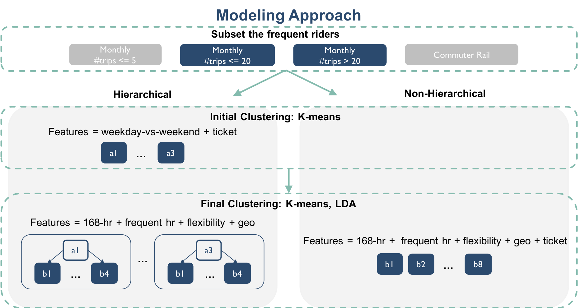
Our overall segmentation approach is summarized in Figure 1.

Figure 1: Segmentation Pipeline

Based on feedback from the client, we first filtered out riders with a commuter rail pass (except for Zone 1a) and riders who ride fewer than 5 trips per month. The rationale is that there is not enough information for performing inference on these riders based on the current fare transaction data collection system.

Recall that our feature sets (details) are:

• 168 Hourly Temporal Patterns: The number of trips each rider took in each hour (0:00 to 23:00) of each day of week (Mon to Sun), a 168-dimensional vector.
• Weekend-vs-Weekday: the total number of trips each rider took on weekday and on weekends.
• Most Frequent Trip Hours: The top 2 hours in which each rider takes most trips during weekdays, and the top 1 hour over weekends.
• Time Flexibility Scores: The maxes of the weekday and weekend ridership distributions.
• Geographical Patterns by Zip Codes: The number of trips each rider took in each zip code.
• Ticket Purchasing Patterns: The number of different service-brands, tariff (e.g., 7-day pass, monthly pass, Pay-as-you-go) and user-type associated with each rider ID.

Our modeling structure offers several functional options for the users to choose. We discuss these options below.

User-Specified Options

Pipeline Options

We implemented two clustering pipelines:

• The Non-hierarchical pipeline is the more conventional pipeline where the user-specified algorithm is directly applied to a set of features. In this case, the set of features is 168 hourly temporal patterns, most frequent trip hours, time flexibility scores, geographical patterns by zip codes and ticket purchasing patterns.
• The Hierarchical pipeline is a custom pipeline where we first used K-means to cluster based on “higher-level” usage patterns, which we defined as the set of weekend-vs-weekday and ticket purchasing patterns (The initial clustering step). The resulting clusters are then clustered again using user-specified algorithm based on more specific features, which we defined as the set of 168 hourly temporal patterns, most frequent trip hours, time flexibility scores and geographical patterns by zip codes (The final clustering step).

To optimize the number of clusters at each clustering step (initial and final), we used the Calinski and Harabaz score, which is defined as the ratio between the within-cluster dispersion and the between-cluster dispersion. For more information on this scoring criterion, please consult the Sklearn documentation on Calinski Harabaz Score.

Algorithm Options

We implemented two unsupervised clustering algorithms for the user to choose and compare:

• Latent Dirichlet Allocation (LDA) - Briefly, LDA learns a mixture distribution of K topics (K is set as a priori) from a set of documents, where a document in our case represent an individual rider and a topic represents a rider-type (e.g., more/less flexible commuter, weekend rider, random rider and etc.). With LDA, each rider is modeled as a distribution of probabilities for being in each rider-type. For more information, refer to Sklearn documentation on LDA.
• K-means - Briefly, K-means clusters data by trying to separate samples in n groups of equal variance, minimizing a criterion known as the inertia or within-cluster sum-of-squares. For more information, refer to Sklearn documentation on K-means.

Options for Feature Weights

Since policy makers might wish to develop policies targeting a certain aspect of rider behavior (e.g. time of use vs. location of use), our package allows flexibility in weighting different feature sets. Recall that we roughly divided our feature sets into 3 broad categories: temporal, geographical and ticket purchasing patterns. The segmentation module in the package takes in a single user-specified value for weights on the temporal patterns (w, from 0 to 100), and the two different pipelines handles this user input differently.

With the non-hierarchical pipeline:

Step	Feature Set	Weight
Final Clustering	168 Hourly Temporal Patterns + Most Frequent Trip Hours + Time Flexibility Scores	w
	Geographical Patterns by Zip Codes	0.5(100 - w)
	Ticket Purchasing Patterns	0.5(100 - w)

With the hierarchical pipeline:

Step	Feature Set	Weight
Initial Clustering	Weekend-vs-Weekday	100
	Ticket Purchasing Pattern	100
Final Clustering	168 Hourly Temporal Patterns + Most Frequent Trip Hours + Time Flexibility Scores	w
	Geographical Patterns by Zip Codes	100 - w

Summary Findings

• Hierarchical vs. Non-Hierarchical Pipeline: The hierarchical pipeline appears to have 2 advantages over the non-hierarchical pipeline - 1) More time efficient; and 2) Able to find clusters with more subtle differences
• LDA vs. K-means: LDA produces clusters with better size stability and more interesting subtle differences than K-means. K-means tends to pick up very small rider segments that have very distinct usage patterns.